Indexology^® Blog

Rates, volatility and a broad market rally have contributed to the factor’s late-summer slump

Late summer has not been fruitful for the low volatility factor. From July 6 to Sept. 9, the S&P 500 Low Volatility Index has fallen by 4.67%, while the S&P 500 Index gained 1.70%.¹ This is in sharp contrast to the second quarter, when the low volatility index returned 6.75%, and the broad-market index returned 2.46%.¹ Naturally, some investors are wondering what’s behind the shift.

Looking at market conditions during this time, I see three headwinds that were working against the low volatility factor:

• Interest rates rose. The 10-year Treasury yield rose from 1.31% on July 6 to a close of 1.67% on Sept. 9.¹
• Volatility was relatively flat. The CBOE Volatility Index (the VIX) was 14.96 on July 6 and was 12.51 on Sept. 8. before finishing at 17.5 on Sept. 9.¹
• The S&P 500 Index rallied. While the index gave back much of its earlier gains on Sept. 9, it had rallied for most of July and August.

When has low volatility outperformed?
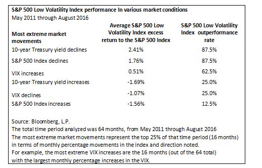
The low volatility factor has tended to shine when interest rates are flat to lower, stock prices are falling and volatility is rising.  We can see this in the table below, which examines the performance of the S&P 500 Low Volatility Index during extreme moves in the S&P 500 Index, the VIX and 10-year Treasury yields from May 2011 through August 2016. In that time frame, there were 64 months of returns. The table examines low volatility performance during the most extreme months (the top 25%) in terms of the largest increases and decreases in each index.

Examining low volatility results

• By volatility. During the 16 months when the VIX had its largest percentage increases, the S&P 500 Low Volatility Index outperformed the S&P 500 Index 62.5% of the time, with an excess return of 51 basis points (bps). In contrast, during the 16 months when the VIX had its largest percentage drops, the low volatility index outperformed the broad market just 25% of the time, with an average lag of 107 bps.
• By rates. During the 16 months when the 10-year Treasury yield had its largest percentage increases, the S&P 500 Low Volatility Index outperformed the S&P 500 Index just 25% of the time, trailing by an average of 169 bps. During the top months of yield declines, the low volatility index outperformed the broad market 87.5% of the time, with an average excess return of 241 bps.
• By market performance. During the 16 months when the S&P 500 Index had its largest declines, the S&P 500 Low Volatility Index outperformed 87.5% of the time, with an average excess return of 176 bps. In contrast, during months when the S&P 500 Index gained the most, the low volatility index outperformed 12.5% of the time, with an average underperformance of 156 bps.

Bottom line: Low volatility is performing as expected|
When you look at the market conditions experienced in late summer, it’s no surprise that low volatility shares underperformed the broad market. This is by design. However, it’s important to remember that the low volatility factor does occasionally outperform in up markets and occasionally lag in down markets.  And while higher rates and a lower VIX have been headwinds for low volatility, the results are not absolute. There are exceptions. Understanding market trends and the potential for exceptions can help investors set proper expectations for low volatility performance.

In my last post, I discussed variability in cost and affordability of retirement income.  I used some data from S&P STRIDE, our new benchmark that provides a cradle-to-grave yardstick for wealth accumulation and income generation.  This week, I will look a little closer at how we measure retirement income, as well as its present value or cost.  To begin with, defined contribution retirement plan participants and IRA investors must convert their accumulated savings into an income stream when they enter retirement.  Things may be simpler for people with defined-benefit pensions that pay out monthly benefits according to the plan’s vesting schedule and benefit formula.  However, even though defined benefits are expressed as monthly income, they have a present value, which is simply the stream of their expected future cash flows expressed as a discounted lump sum.

If you were to ask people of my parent’s generation, “What is your net worth?” they probably would not count the present value of their pension benefits.  They may view it as part of their personal income statement but not their balance sheet.  However, if you asked people in my generation the same question, I bet they would include the value of their 401(k).  They are thinking of it as a balance sheet item, but many have not yet considered that it needs to become an income statement item upon retirement.

When considering the convertibility of lump sums into income streams and vice versa, it may help to think about how the bond market works.  When you buy a bond, you convert a given amount of liquid funds into future cash flows, and when you sell a bond, you convert future cash flows into readily available capital.  As we know, bond prices vary with interest rates, and the same applies to future retirement income.  The bond market analogy is relevant because at S&P DJI, we calculate the value of retirement income exactly like the value of a bond.  However, we define a special “bond” called the generalized retirement income liability (GRIL) as a particular set of cash flows.  Specifically, GRIL is defined as USD 1 per year of inflation-adjusted income starting at age 65 and continuing for 25 years.  We discount GRIL’s cash flows using the U.S. Treasury Inflation-Protected Securities (TIPS) yield curve.  This results in a transparent, precise method for evaluating the cost of future inflation-adjusted (real) income.  We calculate the present value of GRIL for various starting points, each corresponding to specific target years within the S&P STRIDE Indices.  Currently, they range from 2005 to 2060.  For example, if you plan to retire around 2035, you can find the cost of retirement income as we calculate it on our website under the “additional info” menu.  Exhibit 1 shows the cost of 2035 GRIL since January 2016:

What does Exhibit 1 tell us?  GRIL is 25 US dollars of inflation-adjusted retirement income spread over 25 years—USD 1 per year.  To buy that income stream at the end of January 2016 would have cost USD 17.40, but as of September 2016, its cost increased to USD 20.68.  Therefore if you held $1 million in US T-Bills (potentially the safest investment one can find, from the perspective of investment volatility), in January 2016, you could have acquired $57,471 of today’s US dollars per year starting in 2035 and lasting until 2060.  The calculation is USD 1 million / USD 17.40.  However, because real interest rates trended down since the start of the year, increasing the cost of income, as of September 2016 that same $1 million T-Bill portfolio would only have bought $48,356 of future income (USD 1 million / USD 20.68).  When viewed through the lens of income affordability, it is therefore clear that investing in T-Bills and other short-term obligations is not risk free.

The annual rebalancing of the Dow Jones Sustainability Indices (DJSI), the most famous benchmark for corporate sustainability in the world, took place on September 8^th 2016. With nearly 2,000 companies analyzed currently and another nearly 2,000 to be analyzed in RobecoSAM’s 2016 Corporate Sustainability Assessment (CSA), it is clear that sustainability is no longer something “nice to have,” but rather a necessity in order to remain cutting-edge. Likewise, the growing number of requests for new indices proves that there is appetite for fresh products among investors. At the core of this positive trend is the recognition that long-term sustainability factors are the key to long-term value creation. This has set the stage for exciting new developments.

S&P Long-Term Value Creation Index
RobecoSAM had the opportunity to work together with the Canada Pension Plan Investment Board (CPPIB) a leading supporter of the long-term investing movement. The belief that sustainability is by definition something that can and will play out over a long time horizon also attracted the interest of S&P Dow Jones Indices. The result was the S&P Long-Term Value Creation Index, an innovative product that has garnered much investor attention. This index focuses not only on the long-term financial viability of a company, but also on its sustainability performance.

New questions
RobecoSAM introduced a number of new questions to its CSA in 2016, including questions on the sources of long-term value creation, how goals are aligned with remuneration, and how transparent companies are in discussing progress towards sustainability goals. These new questions, found within the new “Materiality” criterion, were the product of discussions about what the sources of long-term management creation really are.

Impact measurement
Another area of development in this year’s CSA was impact measurement. While the term has gained traction within the investment community, impact measurement is often backward-looking. Thus, the “Impact Measurement & Valuation” criterion introduced in the CSA rests on major global drivers such as the United Nations Sustainable Development Goals (SDGs). These goals provide companies and investors with a compass to steer their sustainability initiatives towards global challenges. RobecoSAM regards these goals as essential for companies to ensure that they are generating value for all stakeholders. As investors also begin to align their strategies towards the UN SDG’s, companies that can demonstrate they are thinking long-term will have the upper-hand.

Conclusion
Looking back over 2016, we can see that progress has been made to encourage long-term strategies among companies and investors. But more work needs to be done. With new products like the S&P Long-Term Value Creation Index, the JPX/S&P CAPEX & Human Capital Index, the S&P DJI Fossil-Fuel Free index series and the Dow Jones Sustainability Indices, we have taken steps towards offering investment opportunities focused on long-term sustainability themes. RobecoSAM believes that creating long-term value and solving the world’s biggest sustainability challenges are not things that should be tackled in isolation, but rather tackled at both ends, where investors and companies each do their part to ensure a viable future.

Legal Information: The information and opinions contained in this publication constitutes neither a solicitation, nor a recommendation, nor an offer to buy or sell investment instruments or other services, or to engage in any other kind of transaction. RobecoSAM AG and its related, affiliated and subsidiary companies disclaim all warranties, expressed or implied, including, but not limited to, implied warranties of merchantability and fitness for a particular purpose. In no event shall RobecoSAM AG and its related, affiliated and subsidiary companies be liable for any direct, indirect, special, incidental or consequential damages arising out of the use of any opinion or information expressly or implicitly contained in this publication. © 2016 RobecoSAM AG.

There are many in the healthcare market who have speculated that the Affordable Care Act (ACA) was doomed to fail due to high-cost individuals with pre-existing conditions driving up the average cost of care, while the healthy population that needed to support the cost of care for the sick remained on the sidelines with little-to-no incentives to become insured.  The S&P Healthcare Claims Indices supported this theory throughout 2015, when the average cost of care for a patient with an individual health insurance policy topped out at USD 415.15 versus USD 388.70 for an employee covered under an ASO type policy by their employer, or USD 338.92 for an employee covered under a large group type policy by their employer (see Exhibit 1).  That is, USD 26.45 more to treat a patient covered by an individual policy versus a self-insured type policy, and a whopping USD 76.23 more to cover an individual policy patient versus a patient covered by a large group policy by their employer.  Under both the self-insured and large group structure, the employer requires all employees to maintain insurance, which in effect forces a suitable population of healthy people to pay for unhealthy people.

What Has Changed?

As seen in Exhibit 1, we can see a drop in the average cost of care for a patient covered under an individual policy starting in 2016.  Now that costs for individual policies are in line with those of employers, one can argue that this is how the ACA was envisioned to work.  With everybody having access to care, everybody paying their fair share, average costs should be in line with that of the overall market.  However, a more in-depth study is needed to understand the reasoning behind individual policy costs coming in line with the employer market.  We envision several potential reasons for the larger drop in average costs relative to the employer market.  In this edition, we will focus on one possible explanation.

When plan enrollees approach the end of a plan year, they often review their total out of pocket costs for that given year.  In a year where plan members have hit their maximum out of pocket costs, they are more likely to continue to spend and try to get all elective health issues addressed in the current year rather than carry them over to the next plan year where their maximum out of pocket costs will reset.  If we think about how the ACA enticed many uninsured individuals with pre-existing conditions to enter the market, buy insurance, and utilize that coverage to address their existing needs, it only makes sense that they will try to address all of their pre-existing conditions in the same plan year to avoid unnecessary out of pocket expenses.  If this is the case, then 2015 should be an anomaly, and moving forward we should see average individual costs stay in line with employer costs, assuming the ACA is working the way it was intended to work.

We all know we should work on and improve our core, but how many of us have the discipline to do it?  I interviewed two financial advisors who are strengthening their core by using municipal bond indices and the ETFs that track them.

Matt Papazian is founding partner and CIO at Cardan Capital Partners of Denver, Colorado, and Tom Cartee is a financial advisor and portfolio manager at Sheets Smith Wealth Management of Winston-Salem, North Carolina.

S&P DJI: Has the availability of indices or beta for municipal bonds changed the way that you are able to use municipal bonds?

Matt: Yes.  The ability to move weightings seamlessly between credit and duration is a great benefit of these new offerings.  We are now able to access the high-yield municipal bond space with ease, something we would not normally do with individual bonds.  Because of the historically low default rate in the municipal bond space, including high-yield bonds, we view access to different segments of the municipal bond market as an integral part of how we invest.

Tom: I agree with Matt.  I like to use equity ETFs based on broad indices as the core building blocks of client portfolios.  Municipal bond ETFs enable me to use a similar low-cost, broadly diversified approach to fixed-income allocation within taxable accounts.

S&P DJI: We’ve observed robo-advisors using core municipal bond ETFs within even the most basic asset allocations and at every level of client investment.  Are you finding it easier to deliver this asset class to the smaller clients you work with?

Matt: For smaller market participants, ETFs provide a substantially more efficient way to invest in tax-free bonds.  Small trades in bonds are generally quite expensive for small market participants, even if they don’t see the fee, so ETFs have leveled the playing field for them.

Tom: Trading small lots of individual municipal bonds is not very efficient.  The liquidity available with municipal bond ETFs offers a compelling reason to emphasize ETFs over individual bonds in smaller accounts.

S&P DJI: What are your thoughts on combining index-based municipal bonds with individual municipal bonds?

Matt: Although the majority of our municipal bond investing is done with ETFs, we view individual bonds as a valid way to get exposure to the space for larger investors, but we prefer ETFs for their liquidity and low transaction cost.  We also avail ourselves of closed-end funds when the values are compelling.

Tom: Again, I agree with Matt.  ETFs offer many advantages.  Because tax rates vary from state to state and liquidity needs vary among market participants, advisors may decide to use municipal bond ETFs alongside individual bonds in certain accounts.  The key is to recognize that municipal bond ETFs can be the core, given their favorable characteristics.

My thanks to Matt and Tom for participating in this interview and in a recent webinar on core municipal bond investing that is now available in our webinar archive.